Tips for Formatting A Lot of GWAS Summary Association Statistics Data
By Huwenbo Shi, February 2nd, 2018, see original post @Huwenbo
Summary
Publicly available GWAS summary association statistics data are in all kinds of formats. The diversity of data formats is often attributable to the nature of the phenotypes being studied (e.g. case-control trait / quantitative traits) and the software used to perform the analysis. However, before any post-GWAS analyses, one needs to convert data in various formats into the same format. This page aims to provide some tips, guidelines, and protocols that I find useful for formatting a lot of GWAS summary statistics data to help prevent pitfalls in post-GWAS analyses.
Step 0 – Rename, Date, and Record the Publication of the Data
GWAS summary stats data files often come with file names that are also all over the place. Before looking into the details of the data, we recommend to come up with an abbreviation for the phenotype, and rename the files in a consistent fashion. This will make your life a lot easier in the long run. For example, for the 2014 schizophrenia GWAS summary stats data, the file name could be SCZ_2014.txt, and for the 2014 rheumatoid arthritis GWASs in multiple populations, one could rename the files as RA_ASN_2014.txt, RA_EURO_2014.txt, and A_TE_2014.txt, where TE stands for transethnic. With each GWAS summary stats data, we also recommend to include a readme document to record the publication of the GWAS summary data, and the URL the data was downloaded from. And the file names of the readme document could be something like SCZ_2014.readme. Lastly, we recommend to store all the readme files and freshly downloaded summary stats files in a folder called 0_Raw.
Step 1 – Take A Look at the Header and Figure Out What’s Missing
The header of GWAS summary statistics data files tells what type of information of the GWAS is available and unavailable in the file. The following is a list of some typical headers. If the information that one need for their analyses is not in the header (e.g. sample size, number of cases and controls, etc.), then one will have to read the GWAS paper to extract these information.
snp effect_allele other_allele maf effect stderr pvalue
snpid hg18chr bp a1 a2 zscore pval CEUmaf
SNPID CHR POS A1 A2 Freq_HapMap Zscore Pvalue
Chromosome Position MarkerName Effect_allele Non_Effect_allele Beta SE Pvalue
Marker Chrom Pos Allele1 Allele2 Ncases Ncontrols GC.Pvalue Overall
SNPID CHR BP Allele1 Allele2 Freq1 Effect StdErr P.value TotalN
SNP CHR BP A1 A2 OR SE P INFO EUR_FRQ
rsID,allele1,allele2,freqA1,beta,se,pval,N
Marker Chr Position PValue OR(MinAllele) LowerOR UpperOR Alleles(Maj>Min)
Chr Position Allele1 Allele2 Freq1 Pvalue EffN
Note on Genome Build
Many freshly downloaded GWAS summary stats also only contain SNP ID and not chromosome number or base pair positions. In some cases, some old GWASs before 2012 use HG18 (NCBI B36) for base pair positions. For these type of data, one has to match the SNP IDs against the reference panel legend to find out the chromosome number and base pair positions.
Note on Sample Size
Note that some GWASs report the total sample size, which includes samples both in the discovery stage, and samples in the replication stage. However, it’s often the case that sample size of the discovery GWAS stage is the one that matches the data.
Step 2 – Create Your Own Headers and Compute the Relevant Information
Most GWAS summary stats data do not come with all the information one needs. For example, it’s very often the case that GWAS summary stats file do not contain Z-scores, but rather effect size (odds ratio for case-control traits) and its standard error, and some GWASs provide p-values and effect size. Since Z-score information is used in many summary-data-based software such as LDSC and HESS, it’s highly recommended to include Z-score information in the formatted summary stats file. In general, it’s highly convenient to always have the following 7 columns in the formatted summary stats file. Other informative information such as allele frequency, number of cases and controls can be appended after the first 7 columns. We recommend to store the processed summary stats files in separate directory named 1_Processed.
- SNP : SNP ID (it’s recommended to only include SNPs with rs IDs in the data, as these SNPs are often more well-characterized)
- CHR : Chromosome number (some GWAS summary data contain SNPs on chromosome X, Y, and MT, but usually these SNPs are filtered out during QC)
- BP : Base pair positions (make sure all formatted summary stats use the same genome build)
- A1 : Effect allele (also sometimes called risk allele, reference allele, effect allele, coded allele, etc.)
- A2 : Non-effect allele (also some times called alternate allele, the other allele etc.)
- Z : Z-score with respect to the effect allele, i.e. if Z-score is positive then the effect allele increases the phenotype
- N – Sample size (this is often the discovery stage sample size, not maximum sample size)
Note on Computing Z-scores
If effect size and standard error are included in the freshly downloaded GWAS summary stats file, then Z-score can be computed as
If odds ratio and standard error are included, then Z-score can be computed as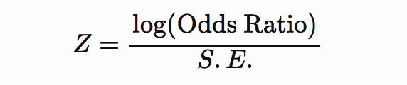
If p-value and effect size (odds ratio) are available then Z-score can be computed as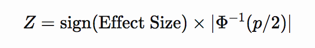
or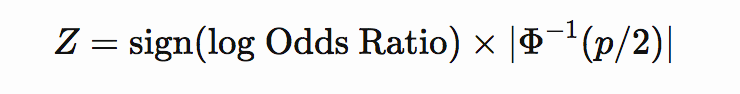
where Φ−1Φ−1 is the inverse cumulative distribution function of the normal distribution.
Step 3 – Quality Control and Align the Alleles Against A Reference Panel
By step 2, all the freshly downloaded GWAS summary stats file should be in a uniform format that is easy to work with. The next step is to perform quality control on the SNPs, i.e. removing SNPs that can screw up your analyses. We recommend to apply the following 8 filtering steps:
- Remove all non-biallelic SNPs
- Remove all SNPs with strand-ambiguous alleles (SNPs with A/T, C/G alleles)
- Removed SNPs without rs IDs, duplicated rs IDs or base pair position.
- Removed SNPs not in 1000 Genomes Project Phase 3 (or any other reference panel that one uses)
- Removed SNPs whose base pair positions or alleles doesn’t match those in 1000GP Phase 3 (or any other reference panel)
- Removed SNPs with imputation INFO less than 0.9 (if INFO is provided)
- Removed all SNPs on chromosome X, Y, and MT
- Removed SNPs with sample size 5 standard deviations away from the mean. (This is to guard against scenarios where some SNPs were genotyped on a specialized genotyping array and have substantial more samples than the rest.)
The results of these step could be stored in a directory named 3_Filtered.
In addition to SNP filtering, it’s also convenient to align the alleles (effect allele and non-effect allele) of each SNP of all processed GWAS summary stats data against those of a referenc panel, so that every GWAS summary stats has the same effect allele, and non-effect allele. In the process, one may need to flip the sign of Z-scores (also effect size, log odds ratio, etc.) if the alleles of a SNP in the summary stats is the reverse of the alleles of the reference panel. For example if a SNP has effect / non-effect alleles as A/G and a Z-score of 1.0 in the summary stats, and effect / non-effect alleles as T/C in the reference panel, then one changes the alleles A/G to T/C and Z-score to -1.0.
Step 4 – Making Sure Everything Is Done Correctly
After step 3, the summary stats file should be good to go with running LDSC. To make sure that the summary stats file are formatted correctly, one could run cross-trait LDSC to see if the genetic correlation between a pair of traits is within expectation. It’s also helpful to have your lab mates go over the pipeline to make sure correctness.
Conclusion
Formatting GWAS summary stats data can be a daunting task given the various kinds of data format out there and the number of pitfalls that can screw up your analysis. This page serves to provide some tips, personal ideas to handle data formatting and help preventing surprises.